
Bioinformatics brings statistics, mathematics, and computer programming to biology and other sciences. In my area, it allows for the analysis of massive amounts of genomic (DNA), transcriptomic (RNA), proteomic (proteins), or metabolomic (metabolites) data.
In recent years, the advances in sequencing have allowed for the large-scale investigation of a variety of microbiomes. Microbiome refers to the collective genetic material or genomes of all the microorganisms in a specific environment, such as the digestive tract or the elbow. The term microbiome is often casually thrown around: some people mistakenly use it interchangeably with “microbiota”, or use it to describe only the genetic material of a specific type of microorganism (i.e. “microbiome” instead of “bacterial microbiome”). Not only have targeted, or amplicon sequencing techniques improved, but methods that use single or multiple whole genomes have become much more efficient. In both cases, this has resulted in more sequences being amplified more times. This creates “sequencing depth”, a.k.a. better “coverage”: if you can sequence one piece of DNA 10 times instead of just once of twice, then you can determine if changes in the sequence are random errors or really there. Unfortunately, faster sequencing techniques usually have more spontaneous errors, so your data are “messy” and harder to deal with. More and messier data creates the problem of handling data.

DNA analysis requires very complex mathematical equations in order to have a standardized way to quantitatively and statistically compare two or two million DNA sequences. For example, you can use equations for estimating entropy (chaos) and estimate how many sequences you might be missing due to sequencing shortcomings based on how homogeneous (similar) or varied your dataset is. If you look at your data in chunks of 100 sequences, and 90 of them are different from each other, then sequencing your dataset again will probably turn up something new. But if 90 are the same, you have likely found nearly all the species in that sample.
Bioinformatics takes these complex equations and uses computer programs to break them down into many simple pieces and automate them. However, the more data you have, the more equations the computer will need to do, and the larger your files will be. Thus, many researchers are limited by how much data they can process.

There are several challenges to analyzing any dataset. The first is assembly.
Sequencing technology can only add so many nucleotide bases to a synthesized sequence before it starts introducing more and more errors, or just stops adding altogether. To combat this increase in errors, DNA or RNA is cut into small fragments, or primers are used to amplify only certain small regions. These pieces can be sequenced from one end to another, or can be sequenced starting at both ends and working towards the middle to create a region of overlap. In that case, to assemble, the computer needs to match up both ends and create one contiguous segment (“contig”). With some platforms, like Illumina, the computer tags each sequence by where on the plate it was, so it knows which forward piece matches which reverse.

When sequencing an entire genome (or many), the pieces are enzymatically cut, or sheared by vibrating them at a certain frequency, and all the pieces are sequenced multiple times. The computer then needs to match the ends up using short pieces of overlap. This can be very resource-intensive for the computer, depending on how many pieces you need to put back together, and whether you have a reference genome for it to use (like the picture on a puzzle box), or whether you are doing it de novo from scratch (putting together a puzzle without a picture, by trial and error, two pieces at a time).

Once assembled into their respective consensus sequences, you need to quality-check the data.
This can take a significant amount of time, depending on how you go about it. It also requires good judgement, and a willingness to re-run the steps with different parameters to see what will happen. An easy and quick way is to have the computer throw out any data below a certain threshold: longer or shorter than what your target sequence length was, ambiguous bases (N) which the computer couldn’t call as a primary nucleotide (A, T, C, or G), or the confidence level (quality score) of the base call was low. These scores are generated by the sequencing machine as a relative measure of how “confident” the base call is, and this roughly translates to potential number of base call errors (ex. marking it an A instead of a T) per 1,000 bases. You can also cut off low-quality pieces, like the very beginning or ends of sequences which tend to sequence poorly and have low quality. This is a great example of where judgement is needed: if you quality-check and trim off low quality bases first, and then assemble, you are likely to have cut off the overlapping ends which end up in the middle of a contig and won’t be able to put the two halves together. If you assemble first, you might end up with a sequence that is low-quality in the middle, or very short if you trim it on the low quality portions. If your run did not sequence well and you have lot of spontaneous errors, you will have to decide whether to work with a lot of poor-quality data, or a small amount of good-quality data leftover after you trim out the rest, or spend the money to try and re-sequence.
There are several steps that I like to add, some of which are necessary and some which are technically optional. One of them is to look for chimeras, which are two sequence pieces that mistakenly got joined together. This happens during the PCR amplification step, often if there is an inconsistent electrical current or other technical problem with the machine. While time- and processor-consuming, chimera checking can remove these fake sequences before you accidentally think you’ve discovered a new species. Your screen might end up looking something like this…

Eventually, you can taxonomically and statistically assess your data.

In order to assign taxonomic identification (ex. genus or species) to a sequence, you need to have a reference database. This is a list of sequences labelled with their taxonomy (ex. Bacillus licheniformis), so that you can match your sequences to the reference and identify what you have. There are several pre-made ones publicly available, but in many cases you need to add to or edit these, and several times I have made my own using available data in online databases.

You can also statistically compare your samples. This can get complicated, but in essence tries to mathematically compare datasets to determine if they are actually different, and if that difference could have happened by chance or not. You can determine if organically-farmed soil contains more diversity than conventionally-farmed soils. Or whether you have enough sequencing coverage, or need to go back and do another run. You can also see trends across the data, for example, whether moose from different geographic locations have similar bacterial diversity to each other (left). Or whether certain species or environmental factors have a positive/negative/ or no correlation (below).

Bioinformatics can be complicated and frustrating, especially because computers are very literal machines and need to have things written in very specific ways to get them to accomplish tasks. They also aren’t very good at telling you what you are doing wrong; sometimes it’s as simple as having a space where it’s not supposed to be. It takes dedication and patience to go back through code to look for minute errors, or to backtrack in an analysis and figure out at which step several thousand sequences disappeared and why. Like any skill, computer science and bioinformatics take time and practice to master. In the end, the interpretation of the data and identifying trends can be really interesting, and it’s really rewarding when you finally manage to get your statistical program to create a particularly complicated graph!
Stay tuned for an in-depth look at my current post-doctoral work with weed management in agriculture and soil microbial diversity!
