I’m counting down the days for my first Ecological Society of America (ESA) conference next week in Portland, OR. Over the last few weeks, I’ve been diligently working to finish as much analysis as possible on the data from my recent post-doc, as I am presenting a poster on Wednesday, August 9th from 4:30 to 6:30 pm; PS 31-13 –Soil bacterial diversity in response to stress from farming system, climate change, weed diversity, and wheat streak virus.
The theme for this year’s ESA meeting is “Linking biodiversity, material cycling and ecosystem services in a changing world”, and judging from the extravagant list of presenting authors, it’s going to be an extremely large meeting. It’s worth remembering that large conferences like these bring together researchers from each rung of the career ladder, and many of the invited speakers will be presenting on work that might have been done by dozens of scientists over decades. Seeing only the polished summary can be intimidating, lots of scientists I’ve spoken to can feel intimidated by these comprehensive meeting talks because the speakers seem so much smarter and more successful than you. It’s something I jokingly refer to as “pipette envy”: when you are at a conference thinking that everyone does cooler science than you. Just remember, someone also deemed your work good enough to present at the same conference!
My greenhouse trial on the legacy effects of farming systems and climate change has concluded! Over this past fall and winter, I maintained a total of 648 pots across three replicate trials (216 trials per). In the past few weeks, we harvested the plants and took various measurements: all-day affairs that required the help of several dedicated undergraduate researchers.
In case you were wondering why research can be so time and labor intensive, over the course of the trials we hand-washed 648 pot tags twice, 648 plant pots twice, planted 7,776 wheat seeds across two conditioning phases, 1,944 wheat seeds and 1,944 pea seeds for the response phase. We counted seedling emergence for those seeds every day for a week after each of the three planting dates in each of the three trials (9 plantings all together). Of those 11,664 plants, we hand-plucked 7,776 seedlings and grew the other 3,888 until harvesting which required watering nearly every day for over four months. At harvest, we counted wheat tillers or pea flowers, as well as weighed the biomass on those 3,888, and measured the height on 1,296 of them. And this is only a side study to the larger field trial I am helping conduct! All told, we have a massive amount of data to process, but we hope to have a manuscript ready by mid-summer – stay tuned!
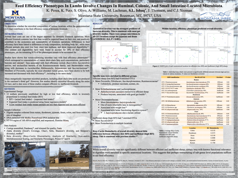
I’m pleased to announce that a paper that I contributed to was recently accepted for publication in the Journal of Animal Science!
“Feed efficiency phenotypes in lambs involve changes in ruminal, colonic, and small intestine-located microbiota”, Katheryn Perea; Katharine Perz; Sarah Olivo; Andrew Williams; Medora Lachman; Suzanne Ishaq; Jennifer Thomson; Carl Yeoman (article here).
Katheryn is an undergraduate at New Mexico Institute of Mining and Technology who received an INBRE grant to support her as a visiting researcher at Montana State University in Bozeman, MT over summer 2016. Here, she worked with Drs. Carl Yeoman and Jennifer Thomson to perform the diversity analysis on the bacteria in the gastrointestinal tract of sheep from a previous study. These sheep had been designated as efficient or inefficient, based on how much feed was needed for them to grow. Efficient sheep were able to grow more with less feed, and it was thought this might be due to hosting different symbiotic bacteria which were better at fermenting fibrous plant material into usable byproducts for the sheep.
Samples from the sheep were collected as part of a larger study on feed efficiency performed by MSU graduate students Kate Perz and Medora Lachman, as well as technicians Sarah Olivo and Andrew Williams, and Katheryn performed the data and statistical analysis using some of my guidelines. This is Katheryn’s first published article, and one I just presented a poster on at the Congress on Gastrointestinal Function in Chicago, IL!
As the 2016 growing season comes to a close in Montana, here in the lab we aren’t preparing to overwinter just yet. In the last few weeks, I have been setting up my first greenhouse trial to expand upon the work we were doing in the field. My ongoing project is to look at changes in microbial diversity in response to climate change. The greenhouse trial will expand on that by looking at the potential legacy effects of soil diversity following climate change, as well as other agricultural factors.
First, though, we had to prep all of our materials, and since we are looking at microbial diversity, we wanted to minimize the potential for microbial influences. This meant that the entire greenhouse bay needed to be cleaned and decontaminated. To mitigate the environmental impact of our research, we washed and reused nearly 700 plant pots and tags in order to reduce the amount of plastic that will end up in the Bozeman landfill.
Each pot needed to be scrubbed with disinfectant soap and then soaked in bleach.
Lines of pots drying on the rack.
I scrubbed 700 labels clean in order to reuse them.
We also needed to autoclave all our soil before we could use it, to make sure we are starting with only the microorganisms we are intentionally putting in. These came directly from my plots in the field study, and are being used as an inoculum, or probiotic, into soil as we grow a new crop of wheat.
This is trial one of three, each of which has three phases, so by the end of 2016 I’ll have cleaned and put soil into 648 pots with 648 tags; planted, harvested, dried and weighed 11,664 plants; and sampled, extracted DNA from, sequenced, and analyzed 330 soil and environmental samples!
Each pot gets six tiny winter wheat seeds planted.
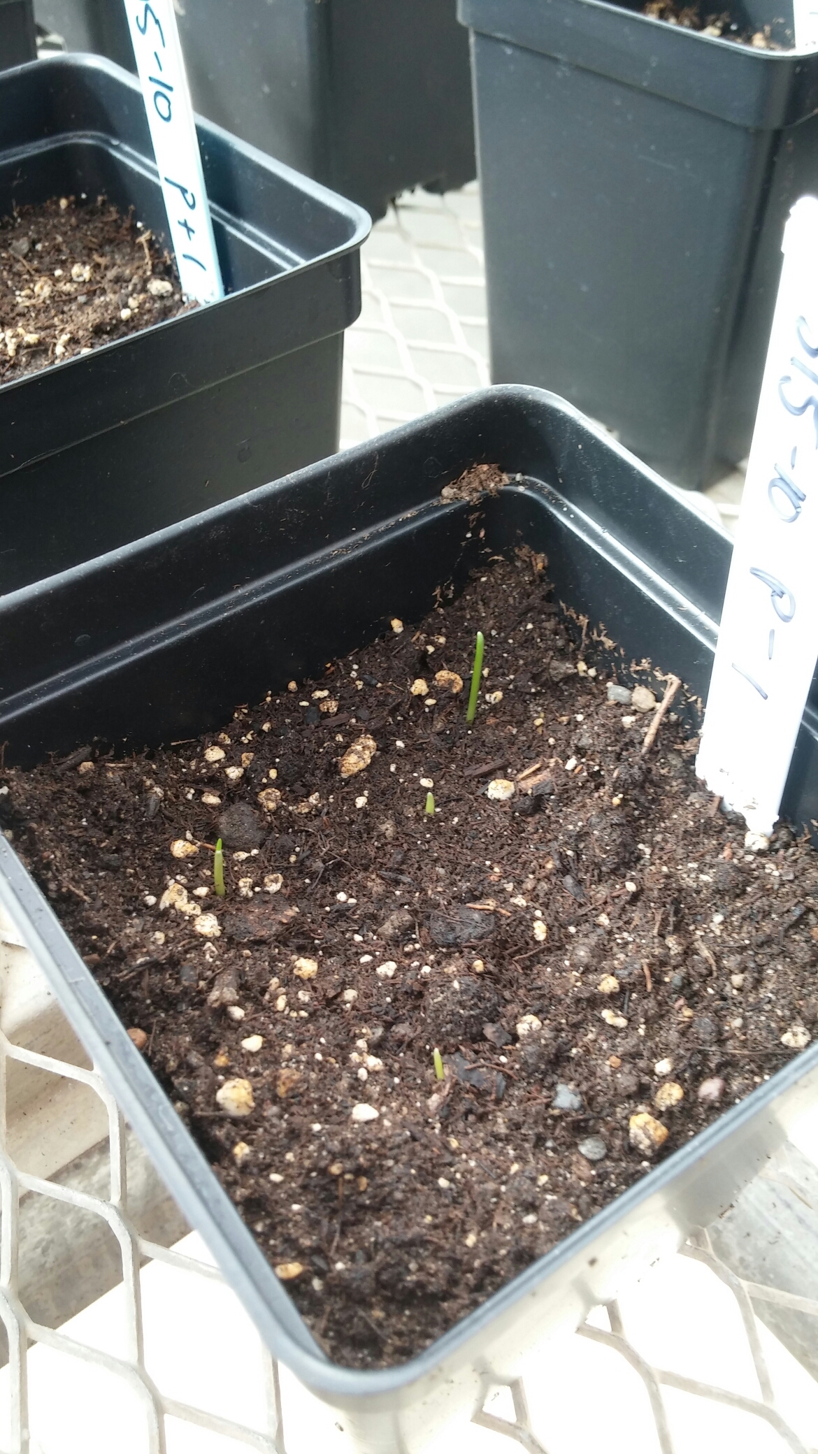
Trial 1: 216 pots ready to grow!
After only a few days, seedlings are beginning to emerge.
Stay tuned for more updates and results (eventually) from this and my field study!
After a hot, dry summer growing season in Montana, the samples have all been collected and the crop harvested for my project investigating wheat production under farming system (organic vs. conventional), climate change (hot or hot and dry), disease (wheat streak virus), and weed competition (cheatgrass) conditions. We collected wheat and weed biomass from every subplot, totaling 108 bags of wheat and an estimated 500 bags of weeds! This will be weighed to determine production, and diversity (number of different weed species) will be assessed.
The biomass bags were temporarily stored in my office until we could find enough shelf space in the lab.
At the end of July, we also collected our final soil samples, which required over 500 grams of aseptically collected of soil in each subplot. With the extremely dry, clay-containing soil on the farm, this was no quick undertaking, and it took 6-7 lab members a total of 9 hours to collect all 108 samples! Those soil samples will be used for DNA sequencing to determine what microorganisms are present, and compared to other time points to see how they changed over the summer in response to our treatment conditions. The soil will also be measured for essential nutrients, such as nitrogen and carbon content, and saved to be used in a greenhouse experiment to look at the legacy effects of microbial change.
The samples might be collected, but we aren’t done yet. This was year one of a two-year project, and as winter wheat and cheatgrass need to be sown soon, before it gets cold, we have a lot of prep work to do. This includes resetting our data collection tools, including gypsum blocks for soil moisture and ibuttons for soil temperature. We will also need to set up our climate chamber equipment in all new subplots, since we are interested in third-year winter wheat that is part of a five-year crop rotation. We also plan to start a greenhouse experiment looking at the legacy effects of our soil this fall. Not to mention all of data to analyze over the winter months!
In May, 2016, I started a post doctoral position in a laboratory that focuses on weed management in agricultural systems, especially organic farms which don’t use chemical fertilizer or herbicide. My role is to integrate microbial ecology. For example, is the soil microorganism diversity different in fields that compete better against weeds than in fields that can’t? Are there certain microorganisms that make it easier for weeds to grow, and how do they do that? Can we suppress weeds by manipulating bacteria or fungi in the soil?
So far, I’ve been doing field work for my project, as well as assisting other lab members in their own projects, as many large scale greenhouse or field experiments require large groups of helpers to accomplish certain tasks. I’m also new to weed ecology, and I wanted to learn as much as possible. Thus, I put on some sunscreen and one of those vendor t-shirts you get when you order a certain dollar amount, and got to work.
Some of our projects investigate the link between crop health and climate change. To simulate climate change, we create rain-out shelters to mimic dry conditions, and plastic shielding to mimic hotter conditions.
Making climate change simulators.
The gypsum block will absorb soil moisture, and we can measure conductivity off of that.
This one is very dry.
One of the treatments is to infect crops with wheat streak mosaic virus, to determine whether climate change will affect the plant’s ability to fight infection, and whether it will change soil microbiota. To do this, we needed to infect our crops, which meant growing infected plants in the laboratory and selectively spreading them in the field as a slurry.
Blended wheat.
We need to filter out the particles or they will clog the sprayer. Also pictured: Dr. Fabian Menalled.
A similar project is using mites as a virus transmission vector, so we attached mite-infected wheat to healthy wheat.
Kyla and I are attaching wheat to other wheat with paperclips.
We hope the wheat mite get infected.
Another project is collecting data about ground beetle diversity in organic versus conventionally farmed soil. For this, we planted pitfalls traps in fields to collect and identify beetles.
Throughout many of the ongoing lab projects, I’ll be investigating the effect of treatments on soil health and diversity.
The core sampler is used to collect soil from certain depths.
The soil is then put in sterile containers until analysis.
My project is part of a larger experiment, which also involves assessing crop and weed communities. For this, we need to randomly sample plants in the field and collect all above-ground plant material (to measure biomass as weight), as well as the biomass of each individual weed species to measure diversity (number of different weed species) and density (how large the plants are actually growing).
This slideshow requires JavaScript.
And, of course, there is plenty of weed species identification!
Field bindweed (Convolvulus arvensis) is an invasive plant related to morning glories. Their winding vines grow into a tangled mass which can strangle other plants, and a single plant can produce hundreds of seeds. The plants can also store nutrients in the roots which allow them to regrow from fragments, thus it can be very difficult to get rid of field bindweed. It will return even after chemical or physical control (tilling or livestock grazing), but it does not tolerate shade very well. Thus, a more competitive crop, such as a taller wheat which will shade out nearby shorter plants, reduce the viability of bindweed.
Bindweed wraps around other plants.
This patch goes all the way to Lazarro.
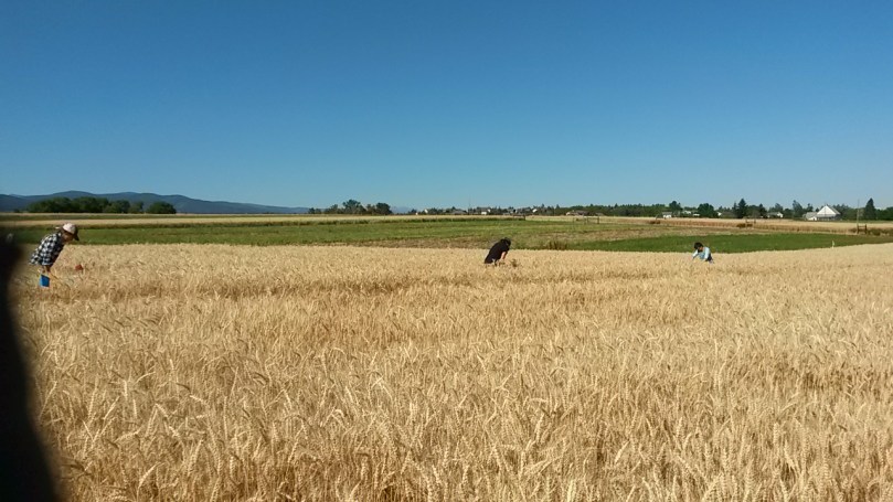
First seen in the US in 1739, Field bindweed is native to the Mediterranean. By 1891, it had made its way west and was identified in Missoula, Montana. As of 2016, it has been reported from all but two counties in Montana, where it has been deemed “noxious” by the state department (meaning that it has been designated as harmful to agriculture (or public health, wildlife, property). In the field, this can be visually striking, as pictured below. In the foreground, MSU graduate student Tessa Scott (lead researcher on this project) is standing in a patch of wheat infested with bindweed. Just seven feet away in the background, undergraduate Lazarro Vinola is standing in non-infested wheat, with soil core samplers used for height reference.
In agricultural fields, bindweed infestations severely inhibit crop growth and health.
Last week, Tessa, Lazarro, and I went to several farms in and around Big Sandy and Lewistown, Montana in order to sample fields battling field bindweed. To do so, we harvested wheat, field bindweed, and other weed biomass by cutting all above-ground plant material inside a harvesting frame. These will be dried and weighed, to measure infestation load and the effect on wheat production.
The sampling locations are consistent with previous years to track how different farm management practices influence infestations. This means using GPS coordinates to hike out to spots in the middle of large fields.
This slideshow requires JavaScript.
It also means getting very dirty driving and walking through dusty fields!
Thalspi, or pennycress, which is dropping seeds even in my shoes!
The van did very well on rocky, uneven field roads!
For the last four days I was in Boston for the American Society for Microbiology (ASM) Microbe 2016 meeting.The meeting is held in Boston on even years, and New Orleans on odd.
The conference brings together all sorts of microbiologists: from earth sciences, to host-associated, to clinical pathologists and epidemiologists, to educators. This year, there were reportedly over 11,000 participants! Because of the wide variety of topics, there is always an interesting lecture going on related to your topic, and it was a wonderful experience to be able to talk directly to other researchers to learn about the clever techniques they are using. I posted about a tiny fraction of those interesting projects on Give Me The Short Version.
On Sunday, I presented a poster on “Farming Systems Modify The Impact Of Inoculum On Soil Microbial Diversity.” I analyzed the data from this project for the Menalled Lab last year, and it has developed into a manuscript in review, as well as several additional projects in development.
One of the best parts of ASM meetings is that you never know who you are going to run into, and I was able to meet up with several friends and colleagues, including Dr. Benoit St-Pierre, who was a post-doc in the Wright lab at the University of Vermont while I was a student, and Laura Cersosimo, the other Ph.D. candidate from the UVM Wright lab who will be defending in just a few months! I also ran into Ph.D. candidate Robert Mugabi, who is hoping to defend by March and in the Barlow lab at UVM while I was there. Most unexpectedly, I ran into a A Lost Microbiologist who had wandered in from Norway: Dr. Nicole Podnecky, who I met at UVM back when we were undergraduates!
This slideshow requires JavaScript.
Of course, no conference would be complete without vendor swag.
Vendor swag! And not even all of it…
Ice cream made using liquid nitrogen from the Witches of Boston.
Bioinformatics brings statistics, mathematics, and computer programming to biology and other sciences. In my area, it allows for the analysis of massive amounts of genomic (DNA), transcriptomic (RNA), proteomic (proteins), or metabolomic (metabolites) data.
In recent years, the advances in sequencing have allowed for the large-scale investigation of a variety of microbiomes. Microbiome refers to the collective genetic material or genomes of all the microorganisms in a specific environment, such as the digestive tract or the elbow. The term microbiome is often casually thrown around: some people mistakenly use it interchangeably with “microbiota”, or use it to describe only the genetic material of a specific type of microorganism (i.e. “microbiome” instead of “bacterial microbiome”). Not only have targeted, or amplicon sequencing techniques improved, but methods that use single or multiple whole genomes have become much more efficient. In both cases, this has resulted in more sequences being amplified more times. This creates “sequencing depth”, a.k.a. better “coverage”: if you can sequence one piece of DNA 10 times instead of just once of twice, then you can determine if changes in the sequence are random errors or really there. Unfortunately, faster sequencing techniques usually have more spontaneous errors, so your data are “messy” and harder to deal with. More and messier data creates the problem of handling data.
The grey lines on the right represent sequence pieces reassembled into a genome, with white showing gaps. The colored lines represent a nucleotide that is different from the reference genome, usually just a random error in one sequence. The red bar shows where each sequence has a nucleotide different from that of the reference genome, indicating that this bacterial strain really is different there. This is a single nucleotide polymorphism (SNP).
DNA analysis requires very complex mathematical equations in order to have a standardized way to quantitatively and statistically compare two or two million DNA sequences. For example, you can use equations for estimating entropy (chaos) and estimate how many sequences you might be missing due to sequencing shortcomings based on how homogeneous (similar) or varied your dataset is. If you look at your data in chunks of 100 sequences, and 90 of them are different from each other, then sequencing your dataset again will probably turn up something new. But if 90 are the same, you have likely found nearly all the species in that sample.
Bioinformatics takes these complex equations and uses computer programs to break them down into many simple pieces and automate them. However, the more data you have, the more equations the computer will need to do, and the larger your files will be. Thus, many researchers are limited by how much data they can process.
Mr. DNA, Jurassic Park (1993)
There are several challenges to analyzing any dataset. The first is assembly.
Sequencing technology can only add so many nucleotide bases to a synthesized sequence before it starts introducing more and more errors, or just stops adding altogether. To combat this increase in errors, DNA or RNA is cut into small fragments, or primers are used to amplify only certain small regions. These pieces can be sequenced from one end to another, or can be sequenced starting at both ends and working towards the middle to create a region of overlap. In that case, to assemble, the computer needs to match up both ends and create one contiguous segment (“contig”). With some platforms, like Illumina, the computer tags each sequence by where on the plate it was, so it knows which forward piece matches which reverse.
When sequencing an entire genome (or many), the pieces are enzymatically cut, or sheared by vibrating them at a certain frequency, and all the pieces are sequenced multiple times. The computer then needs to match the ends up using short pieces of overlap. This can be very resource-intensive for the computer, depending on how many pieces you need to put back together, and whether you have a reference genome for it to use (like the picture on a puzzle box), or whether you are doing it de novo from scratch (putting together a puzzle without a picture, by trial and error, two pieces at a time).
Once assembled into their respective consensus sequences, you need to quality-check the data.
This can take a significant amount of time, depending on how you go about it. It also requires good judgement, and a willingness to re-run the steps with different parameters to see what will happen. An easy and quick way is to have the computer throw out any data below a certain threshold: longer or shorter than what your target sequence length was, ambiguous bases (N) which the computer couldn’t call as a primary nucleotide (A, T, C, or G), or the confidence level (quality score) of the base call was low. These scores are generated by the sequencing machine as a relative measure of how “confident” the base call is, and this roughly translates to potential number of base call errors (ex. marking it an A instead of a T) per 1,000 bases. You can also cut off low-quality pieces, like the very beginning or ends of sequences which tend to sequence poorly and have low quality. This is a great example of where judgement is needed: if you quality-check and trim off low quality bases first, and then assemble, you are likely to have cut off the overlapping ends which end up in the middle of a contig and won’t be able to put the two halves together. If you assemble first, you might end up with a sequence that is low-quality in the middle, or very short if you trim it on the low quality portions. If your run did not sequence well and you have lot of spontaneous errors, you will have to decide whether to work with a lot of poor-quality data, or a small amount of good-quality data leftover after you trim out the rest, or spend the money to try and re-sequence.
There are several steps that I like to add, some of which are necessary and some which are technically optional. One of them is to look for chimeras, which are two sequence pieces that mistakenly got joined together. This happens during the PCR amplification step, often if there is an inconsistent electrical current or other technical problem with the machine. While time- and processor-consuming, chimera checking can remove these fake sequences before you accidentally think you’ve discovered a new species. Your screen might end up looking something like this…
Actual and common screen-shot… but I am familiar enough with it to be able to interpret!
Eventually, you can taxonomically and statistically assess your data.
Ishaq and Wright, 2014, Microbial Ecology
In order to assign taxonomic identification (ex. genus or species) to a sequence, you need to have a reference database. This is a list of sequences labelled with their taxonomy (ex. Bacillus licheniformis), so that you can match your sequences to the reference and identify what you have. There are several pre-made ones publicly available, but in many cases you need to add to or edit these, and several times I have made my own using available data in online databases.
Ishaq and Wright, 2014, Microbial Ecology
You can also statistically compare your samples. This can get complicated, but in essence tries to mathematically compare datasets to determine if they are actually different, and if that difference could have happened by chance or not. You can determine if organically-farmed soil contains more diversity than conventionally-farmed soils. Or whether you have enough sequencing coverage, or need to go back and do another run. You can also see trends across the data, for example, whether moose from different geographic locations have similar bacterial diversity to each other (left). Or whether certain species or environmental factors have a positive/negative/ or no correlation (below).
Bioinformatics can be complicated and frustrating, especially because computers are very literal machines and need to have things written in very specific ways to get them to accomplish tasks. They also aren’t very good at telling you what you are doing wrong; sometimes it’s as simple as having a space where it’s not supposed to be. It takes dedication and patience to go back through code to look for minute errors, or to backtrack in an analysis and figure out at which step several thousand sequences disappeared and why. Like any skill, computer science and bioinformatics take time and practice to master. In the end, the interpretation of the data and identifying trends can be really interesting, and it’s really rewarding when you finally manage to get your statistical program to create a particularly complicated graph!
Stay tuned for an in-depth look at my current post-doctoral work with weed management in agriculture and soil microbial diversity!
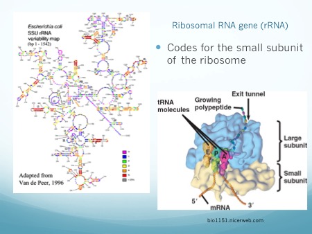
Microbiome studies do not usually employ culturing techniques, and many microorganisms are too recalcitrant to grow in the laboratory. Instead, presumptive identification is made using gene sequence comparisons to known species. The ribosome is an organelle found in all living cells (they are ubiquitous), and it is responsible for translating RNA into amino acid chains. The genes in DNA which encode the parts of the ribosome are great targets for identification-based sequencing. In particular, the small subunit of the ribosome (SSU rRNA) provides a good platform for current molecular methods, although the gene itself does not provide any information about the phenotypic functionality of the organism.
Prokaryotes, such as bacteria and archaea, have a 16S rRNA gene which is approximately 1,600 nucleotide base pairs in length. Eukaryotes, such as protozoa, fungi, plants, animals, etc., have an 18S rRNA gene which is up to 2,300 base pairs in length, depending on the kingdom. In both cases, the 16 or 18 refers to sedimentation rates, and the S stands for Svedberg Units, all-together it is a relative measure of weight and size. Thus, the 18S is larger than the 16S, and would sink faster in water. In both genes, there exist regions which are conserved (identical or near-identical) across taxa, and nine variable regions (V1-V9) [1]. The variable regions are generally found on the exterior of the ribosome, where they are more exposed and prone to higher evolutionary rates. Since the outside of the ribosome is not integral to maintaining its structure, the variable regions are not under functional constraint and may evolve without destroying the ribosome. They provide a means for identification and classification through analysis [2-6]. The conserved areas are targets for primers, as a single primer can bind universally (to all or nearly-all) to its target taxa. The conserved regions are all on the internal structure of the ribosome, and too much change in the sequence will cause its 3D (tertiary) structure to change, thus it won’t be able to interact with the many components in the cell. Mutations or changes in the conserved regions often causes a non-functional ribosome and will kill the cell.
Image: alimetrics.net
In addition to a small subunit, ribosomes also possess a large subunit (LSU rRNA), the 23S rRNA in prokaryotes, and the 28S rRNA in eukaryotes. Eukaryotes have an additional 5.8S subunit which is non-coding, and all small and large units of RNA have associated proteins which aid in structure and function. Taken together, this gives a combined 70S ribosome in prokaryotes, and a combined 80S ribosome rRNA in eukaryotes.
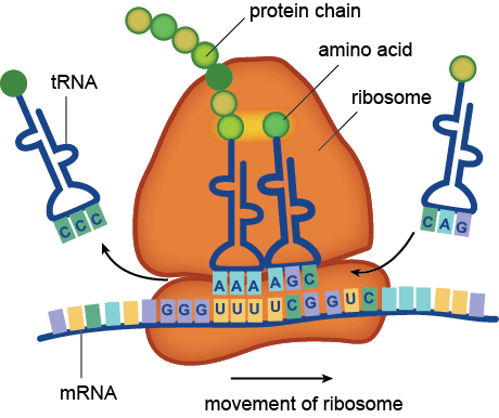
The ribosome assembles amino acids into protein chains based on the instructions of messenger RNA (mRNA) sequences. (Image: shmoop.com)
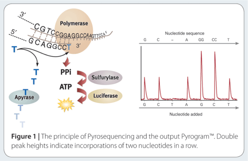
The way to study the rRNA gene is to sequence it. First, you need to extract the DNA from cells, and then you need to make millions of copies of the gene you want using Polymerase Chain Reaction (PCR). PCR and sequencing technology more or less work the same way as a cell would make copies of DNA for cell processes or division (mitosis). You take template DNA, building block nucleotides, and a polymerase enzyme which is responsible for reading the DNA sequence and making an identical copy, and with hours of troubleshooting get a billion copies! Many sequencing machines use nucleotides that have colored dyes attached, and when a nucleotide is added, that dye gets cut (cleaved) off, and the camera can catch and interpret that action. It then records each nucleotide being added to each separate DNA strand, and outputs the sequences for the microorganisms that were in your original sample!
Image: nature.com
The two main challenges facing high-throughput sequencing are in choosing a target for amplification, and being able to integrate the generated data into an increased understanding of the microbiome of the environment being studied. High-throughput sequencing can currently sequence thousands to millions of reads which are up to 600-1000 bases in length, depending on the platform. This has forced studies to choose which variable regions of the rRNA gene to amplify and sequence, and has opened up an arena for debate on which variable region to choose [2]. And of course, the DNA analysis of all this data you’ve now created is quickly being recognized as the most difficult part- which is what I focused on during my post-doc in the Yeoman Lab. Stay tuned for a blog post on the wonderful world of bioinformatics!
Neefs J-M, Van de Peer Y, Hendriks L, De Wachter R: Compilation of small ribosomal subunit RNA sequences. Nucleic Acids Res 1990, 18:2237–2318.
Kim M, Morrison M, Yu Z: Evaluation of different partial 16S rRNA gene sequence regions for phylogenetic analysis of microbiomes.J Microbiol Methods 2010, 84:81–87.
Doud MS, Light M, Gonzalez G, Narasimhan G, Mathee K: Combination of 16S rRNA variable regions provides a detailed analysis of bacterial community dynamics in the lungs of cystic fibrosis patients.Hum. Genomics 2010, 4:147–169.
Yu Z, Morrison M: Comparisons of different hypervariable regions of rrs genes for use in fingerprinting of microbial communities by PCR-denaturing gradient gel electrophoresis.Appl Env Microbiol 2004, 70:4800–4806.
Lane DJ, Pace B, Olsen GJ, Stahl DA, Sogin ML, Pace NR: Rapid determination of 16S ribosomal RNA sequences for phylogenetic analyses.Proc Natl Acad Sci USA 1985, 82:6955–6959.
Yu Z, García-González R, Schanbacher FL, Morrison M: Evaluations of different hypervariable regions of archaeal 16S rRNA genes in profiling of methanogens by archaea-specific PCR and denaturing gradient gel electrophoresis.Appl Env Microbiol 2007, 74:889–893.