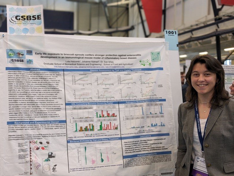
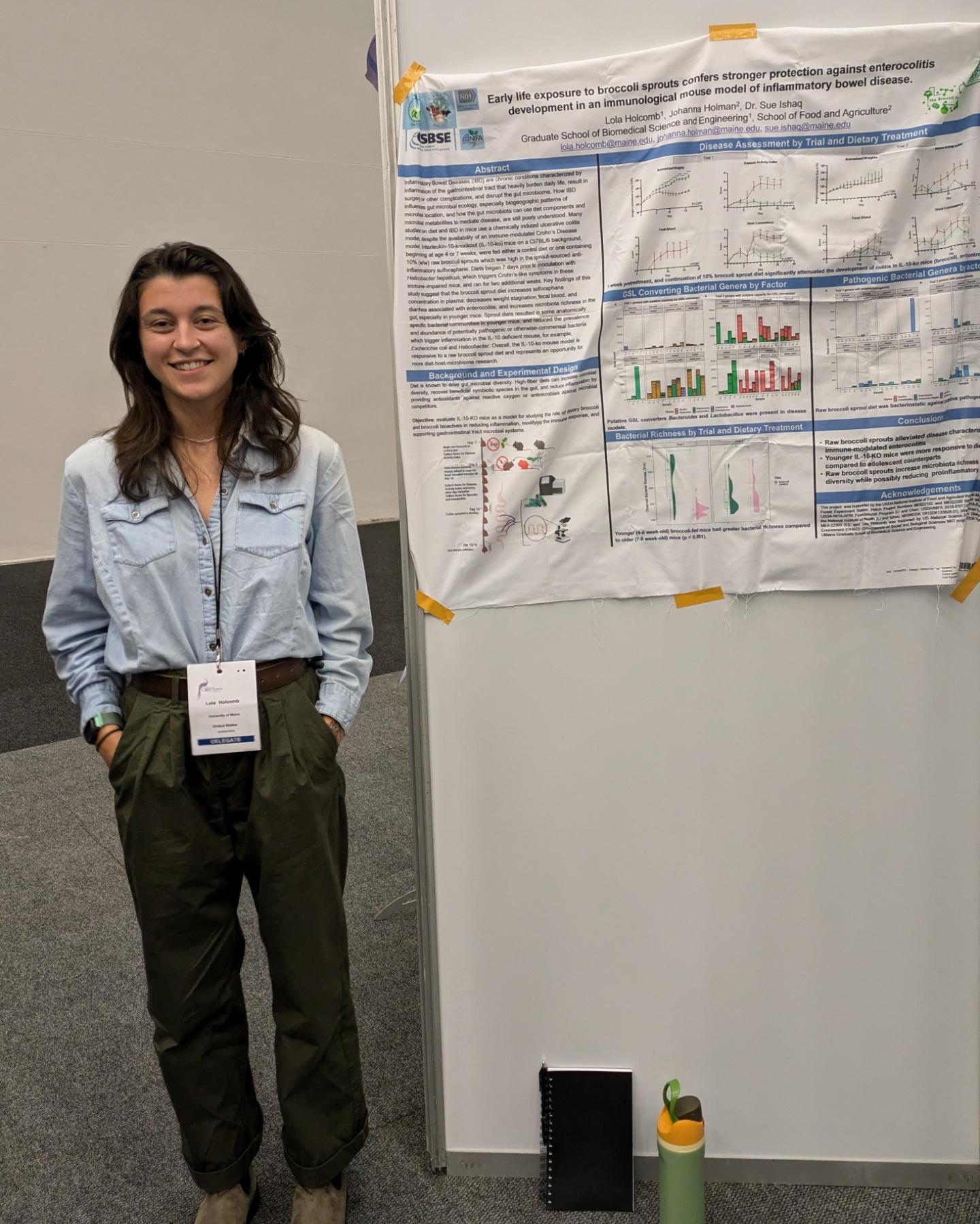
Bioinformatics rockstar, Lola Holcomb, successfully defended her PhD dissertation today on “Anti-Inflammatory Interactions between Gut Microbiota and Broccoli Sprouts”!!!!
Holcomb, Lola. “Anti-Inflammatory Interactions between Gut Microbiota and Broccoli Sprouts”. (2025). University of Maine. Doctor of Philosophy Dissertation (forthcoming). Presentation.
Lola’s contributions to and leadership in the Ishaq Lab Team have led to numerous publications, presentations, and immeasurable professional growth and camaraderie within the group. Her contributions to our research helped us open a new avenue of focus, sparked the imagination of several undergraduates who are now involved in research, and improved the mood and collegiality of the research group with her humor, insightfulness, and poignant questions. Lola has been more of a colleague than a trainee, and the lab is delighted to see how much she’s grown as a researcher. Lola is currently searching for positions as a postdoctoral researcher, bioinformatician, or Assistant Professor at an undergraduate-focused university or college. She’ll continue to collaborate with the Ishaq Lab, as we have multiple manuscripts in review or in preparation for peer review on which she is an author.
Lola entered as a rotating first-year student in March 2022 in the Graduate School of Biomedical Sciences and Engineering program, and declared the Ishaq Lab her dissertation lab soon after, and starting in fall of 2022 was accepted into the NRT funded for One Health in the Environment program. Troubled with indecisiveness and the desire to research, well, everything, she quickly found that using bioinformatics and big data as a lens to study microbial ecology (and in time, its relation to social equity) allowed her to do the kind of meaningful interdisciplinary research she’s always wanted to do. Lola performed 16S data analysis for multiple lab projects and developed a metagenomic analysis workflow to compare gut microbiomes of mouse models of Inflammatory Bowel Disease with broccoli as a dietary treatment. In addition to research, she instructed a graduate-level Genetics course, assisted in Dr. Ishaq’s 16S DNA Sequence Data Analysis course, tutored several Biology undergraduate students, and served as a GSBSE senator in the Graduate Student Government here at UMaine.
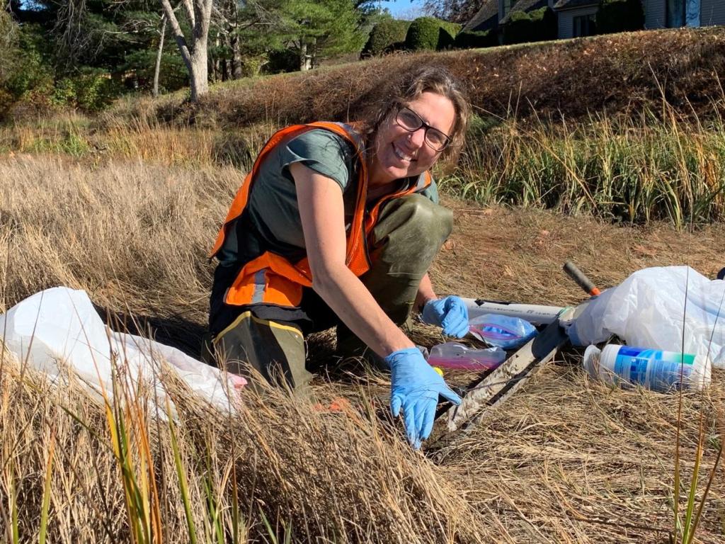
Heather Richard passed her comprehensive exam, which means she is advancing to PhD candidacy!! Heather’s research focuses on how land use and water infrastrucure changes the dynamics of salt marshes and their tidal creeks, which alters their microbial communities, biochemical processes, and capacity to sequester atmospheric carbon in sediment. She details that work, including field sampling and labwork protocols, as well as data visualization and major findings, on an interactive website she created to support research into salt marshes in Maine.
Heather Richard, B.A., M.S.
Doctor of Philosophy Candidate, Ecology and Environmental Sciences. Heather is being co-advised by Dr. Peter Avis
Heather joined the University of Maine in 2021 as a PhD student with the Maine eDNA program and studies the impacts of bridges and roads on microbial communities in salt marsh habitats. Her background in Ecology led her to pursue a career in informal environmental education for several years before getting a Master’s degree in Marine Biology from San Francisco State University studying biofilms on microplastics pollution. Upon returning to Maine in 2016 she led local research for a coastal non-profit organization and has since been dedicated to studying coastal environmental issues relevant to Maine. She has found a true passion in bioinformatic analysis and is eager to learn new tools for data analysis of all kinds.
The exam involved writing mini-papers around topics assigned by her committee, including decision-making and troubleshooting for sequencing data analysis, biogeochemical processes in salt marshes that drive carbon sequestration or release, and microbial ecology in coastal ecosystems. Each set of questions were released once a day for 5 days, and mini-papers took 6 -8 hours to complete and had to be returned within 24 hours. This intensive series of written exams were followed by a two-hour question-and-answer session in which Heather gave further detail on her written answers, connected basic biochemical processes to broader ecosystem-level microbial ecology, and considered furture research designs. This grueling process is the last hurdle for PhD students, and now it’s “smooth sailing” until the PhD defense. Over the next year or so, Heather will perform metegenomics sequencing data analysis from her salt marsh sites, and synthesizing microbial and biochemical data into several manuscripts which we will submit to scientific journals for peer review, and eventual publication.
Sequence data contamination from biological or digital sources can obscure true results and falsely raise one’s hopes. Contamination is a persist issue in microbial ecology, and each experiment faces unique challenges from a myriad of sources, which I have previously discussed. In microbiology, those microscopic stowaways and spurious sequencing errors can be difficult to identify as non-sample contaminants, and collectively they can create large-scale changes to what you think a microbial community looks like.
Samples from large studies are often processed in batches based on how many samples can be processed by certain laboratory equipment, and if these span multiple bottles of reagents, or water-filtration systems, each batch might end up with a unique contamination profile. If your samples are not randomized between batches, and each batch ends up representing a specific time point or a treatment from your experiment, these batch effects can be mistaken for a treatment effect (a.k.a. a false positive).
Due to the high cost of sequencing, and the technical and analytical artistry required for contamination identification and removal, batch effects have long plagued molecular biology and genetics. Only recently have the pathologies of batch effects been revealed in a harsher light, thanks to more sophisticated analysis techniques (examples here and here and here) and projects dedicated to tracking contamination through a laboratory pipeline. To further complicate the issue, sources of and practical responses to contamination in fungal data sets is quite different than that of bacterial data sets.
Chapter 1
“The times were statistically greater than prior time periods, while simultaneously being statistically lesser to prior times, according to longitudinal analysis.”
Over the past year, I analyzed a particularly complex bacterial 16S rRNA gene sequence data set, comprising nearly 600 home dust samples, and about 90 controls. Samples were collected from three climate regions in Oregon, over a span of one year, in which homes were sampled before and approximately six weeks after a home-specific weatherization improvement (treatment homes) or simply six weeks later in (comparison) homes which were eligible for weatherization but did not receive it. As these samples were collected over a span of a year, they were extracted with two different sequencing kits and multiple DNA extraction batches, although all within a short time after collection. The extracted DNA was spread across two sequence runs to allow for data processing to begin on cohort 1, while we waited for cohort 2 homes to be weatherized. Thus, there were a lot of opportunities to introduce technical error or biological contamination that could be conflated with treatment effects.
On top of this, each home was unique, with it’s own human and animal occupants, architectural and interior design, plants, compost, and quirks, and we didn’t ask homeowners to modify their behavior in any way. This was important, as it meant each of the homes – and their microbiomes – are somewhat unique. Therefore I didn’t want to remove sequences which might be contaminants on the basis of low abundance and risk removing microbial community members which were specific to that home. After the typical quality assurance steps to curate and process the data, which can be found on GitHub as an R script of a DADA2 package workflow, I needed to decide what to do with the negative controls.
Because sequencing is expensive, most of the time there is only one negative control included in sequencing library preparation, if that. The negative control is a blank sample – just water, or an unused swab – which does not intentionally contain cells or nucleic acids. Thus anything you find there will have come from contamination. The negative control can be used to normalize the relative abundance numbers – if you find 1,000 sequences in the negative control, which is supposed to have no DNA in it, then you might only continue looking at samples with a certain amount higher than 1,000 sequences. This risks throwing out valid sequences that happen to be rare. Alternatively, you can try to identify the contaminants and remove whole taxa from your data set, risking the complete removal of valid taxa.
I had three types of negative controls: sterile DNA swabs which were processed to check for biological contamination in collection materials, kit controls where a blank extraction was run for each batch of extractions to test for biological contamination in extraction reagents, and PCR negative controls to check for DNA contamination of PCR reagents. In total, 90 control samples were sequenced, giving me unprecedented resolution to deal with contamination. Looking at the total number of sequences before and after my quality-analysis processing, I can see that the number of sequences in my negative controls reduces dramatically; they were low-quality in some way and might be sequencing artifacts. But, an unsatisfactory number remain after QA filtering; these are high-quality and likely come from microbial contamination.
This slideshow requires JavaScript.
I wasn’t sure how I wanted to deal with each type of control. I came up with three approaches, and then looked at unweighted, non-rarefied ordination plots (PCoA) to watch how my axes changed based on important components (factors). What follows is a narrative summarize of what I did, but I included the R script of my phyloseq package workflow and workaround on GitHub.
Chapter 2
“In microbial ecology, preprints are posted on late November nights. The foreboding atmosphere of conflated factors makes everyone uneasy.”
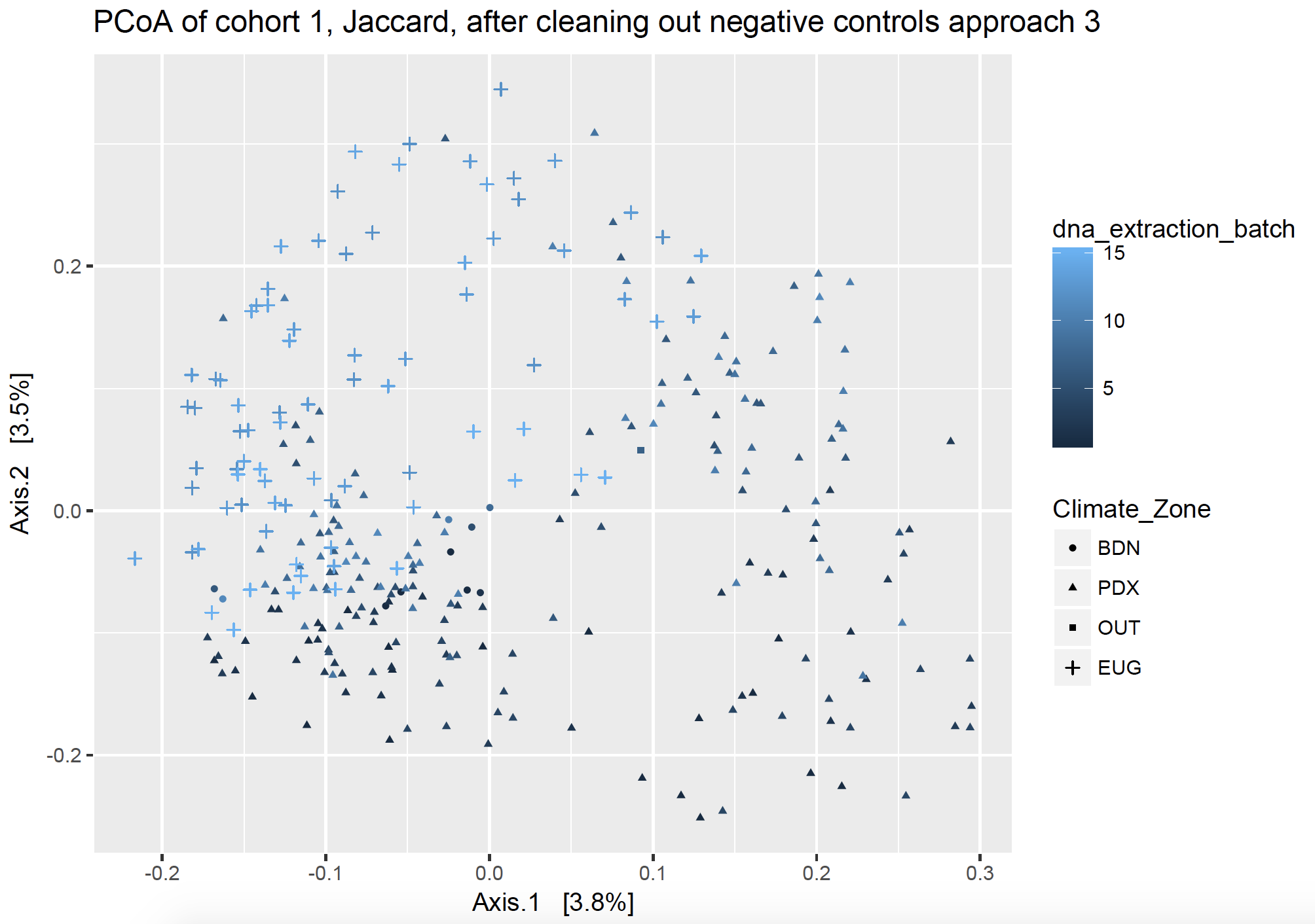
Ordination plots visualize lots of complex communities together. In both ordination figures below, each point on the graph represents a dust sample from one house. They are clustered by community distance: those closer together on the plot have a more similar community than points which are further away from each other. The points are shaped by the location of the samples, including Bend, Eugene, Portland, along with a few pilot samples labeled “Out”, and negative controls which have no location (not pictured but listed as NA). The points are colored by DNA extraction b
Figure 1 Ordination of home samples prior to removing contaminants found in negative controls.
In Figure 1, the primary axis (axis 1) shows a clear clustering of samples by DNA extraction batch, but this is also mixed with geographic location, and as it turns out – date of collection and sequencing run. We know from other studies that geographic location, date of collection, and sequencing batch can all affect the microbial community.
Approach 1: Subtraction + outright removal
This approach subsets my data into DNA extraction batches, and then uses the number of sequences found in the negative controls to subtract out sequences from my dust samples. This assumes that if a particular sequence showed up 10 times in my negative control, but 50 times in my dust samples, that only 40 of those in my dust sample were real. For each of my DNA extraction batch negative control samples, I obtained the sum of each potential contaminant that I found there, and then subtracted those sums from the same sequence columns in my dust samples.
Figure 2 Ordination of home samples after removing contaminants found in negative controls, particular to each batch, using approach 1.
Approach 1 was alright, but there was still an effect of DNA extraction batch (indicated by color scale) that was stronger than location or treatment (not included on this graph). This approach is also more pertinent for working with OTUs, or situations where you wouldn’t want to remove the whole OTU, just subtract out a certain number sequences from specific columns. There is currently no way to do that just from phyloseq, so I made a work-around (see the GitHub page). However, using DADA2 gives you Sequence Variants, which are more precise and I found it’s better to remove them with approach 3.
Approach 2: Total Removal
This approach removes any contaminant sequences that is found in ANY of the negative controls from ALL the house samples, regardless of which negative control was for which extraction batch. This approach assumes that if it a sequence was found as a contaminant in a negative control somewhere, that it is a contaminant everywhere.
Figure 3 Ordination of home samples after removing contaminants found in negative controls, particular to each batch, using approach 2.
Once again, approach 2 was alright, and now that primary axis (axis 1) of potential batch effect is now my secondary axis; so there is still an effect of DNA extraction batch (indicated by color scale) but it is weaker. When I recolor by different variables, there is much more clustering by Treatment than by any batch effects. However, that second axis is also one of my time variables, so don’t want to get rid of all of the variation on that axis. But, since my negative kit controls showed a lot of variation in number and types of taxa, I don’t want to remove everything found there from all samples indiscriminately.
Additionally, I don’t favor throwing sequences out just because they were a contaminant somewhere, particularly for dust samples. Contamination can be situational, particularly if a microbe is found in the local air or water supply and would be legitimately found in house dust but would have also accidentally gotten into the extraction process.
Approach 3: “To each its own”
This approach removes all the sequences from PCR and swab contaminant SVs fully from each cohort, respectively, and removes extraction kit contaminants fully from each DNA extraction batch, respectively. I took all the sequences of the SVs found in my dust samples and made them into a vector (list), and then I took all the sequences of the SVs found in my controls and made them into a different vector. I effectively subtracted out the contaminant SVs by name, but asking to find the sequences which were different between my two lists (thus returning the sequences which were in my dust samples but not in my control samples). I did this respective to each sequencing cohort and batch, so that I only remove the pertinent sequences (ex. using kit control 1 to subtract from DNA extraction batch 1).
Figure 4 Ordination of home samples after removing contaminants found in negative controls, particular to each batch, using approach 3.
In Figure 4, potential batch effect is solidly my secondary axis and not the primary driving force behind clustering. The primary axis (axis 1) shows a clear separation by climate zone, or location of homes, once the batch contamination has been removed. When I recolor by different variables, there is much more clustering by Treatment and almost none by batch effects. I say almost none, because some of my DNA extraction batches also happen to be Treatment batches, as they represent a subset of samples from a different location. Thus, I can’t tell if those samples cluster separately solely because of location or also because of batch effect. However, I am satisfied with the results and ready to move on.
Unlike its namesake, this tale has a happier ending.
To study DNA or RNA, there are a number of “wet-lab” (laboratory) and “dry-lab” (analysis) steps which are required to access the genetic code from inside cells, polish it to a high-sheen such that the delicate technology we rely on can use it, and then make sense of it all. Destructive enzymes must be removed, one strand of DNA must be turned into millions of strands so that collectively they create a measurable signal for sequencing, and contamination must be removed. Yet, what constitutes contamination, and when or how to deal with it, remains an actively debated topic in science. Major contamination sources include human handlers, non-sterile laboratory materials, other samples during processing, and artificial generation due to technological quirks.
Contamination from human handlers
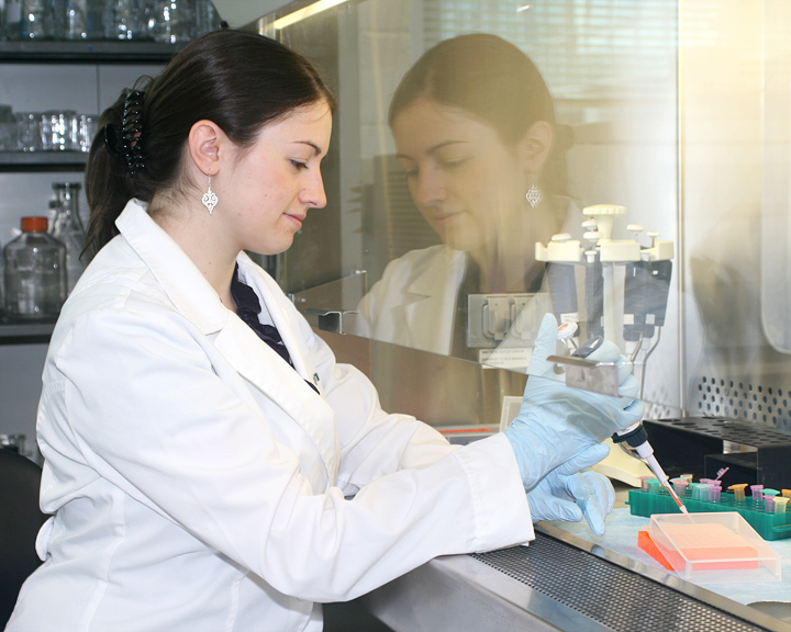
This one is easiest to understand; we constantly shed microorganisms and our own cells and these aerosolized cells may fall into samples during collection or processing. This might be of minimal concern working with feces, where the sheer number of microbial cells in a single teaspoon swamp the number that you might have shed into it, or it may be of vital concern when investigating house dust which not only has comparatively few cells and little diversity, but is also expected to have a large amount of human-associated microorganisms present. To combat this, researchers wear personal protective equipment (PPE) which protects you from your samples and your samples from you, and work in biosafety cabinets which use laminar air flow to prevent your microbial cloud from floating onto your workstation and samples.
Fun fact, many photos in laboratories are staged, including this one, of me as a grad student. I’m just pretending to work. Reflective surfaces, lighting, cramped spaces, busy scenes, and difficulty in positioning oneself makes “action shots” difficult. That’s why many lab photos are staged, and often lack PPE.
Photo Credit: Kristina Drobny
Contamination from laboratory materials
Microbiology or molecular biology laboratory materials are sterilized before and between uses, perhaps using chemicals (ex. 70% ethanol), an ultraviolet lamp, or autoclaving which combines heat and pressure to destroy, and which can be used to sterilize liquids, biological material, clothing, metal, some plastics, etc. However, microorganisms can be tough – really tough, and can sometimes survive the harsh cleaning protocols we use. Or, their DNA can survive, and get picked up by sequencing techniques that don’t discriminate between live and dead cellular DNA.
In addition to careful adherence to protocols, some of this biologically-sourced contamination can be handled in analysis. A survey of human cell RNA sequence libraries found widespread contamination by bacterial RNA, which was attributed to environmental contamination. The paper includes an interesting discussion on how to correct this bioinformatically, as well as a perspective on contamination. Likewise, you can simply remove sequences belonging to certain taxa during quality control steps in sequence processing. There are a number of hardy bacteria that have been commonly found in laboratory reagents and are considered contaminants, the trouble is that many of these are also found in the environment, and in certain cases may be real community members. Should one throw the Bradyrhizobium out with the laboratory water bath?
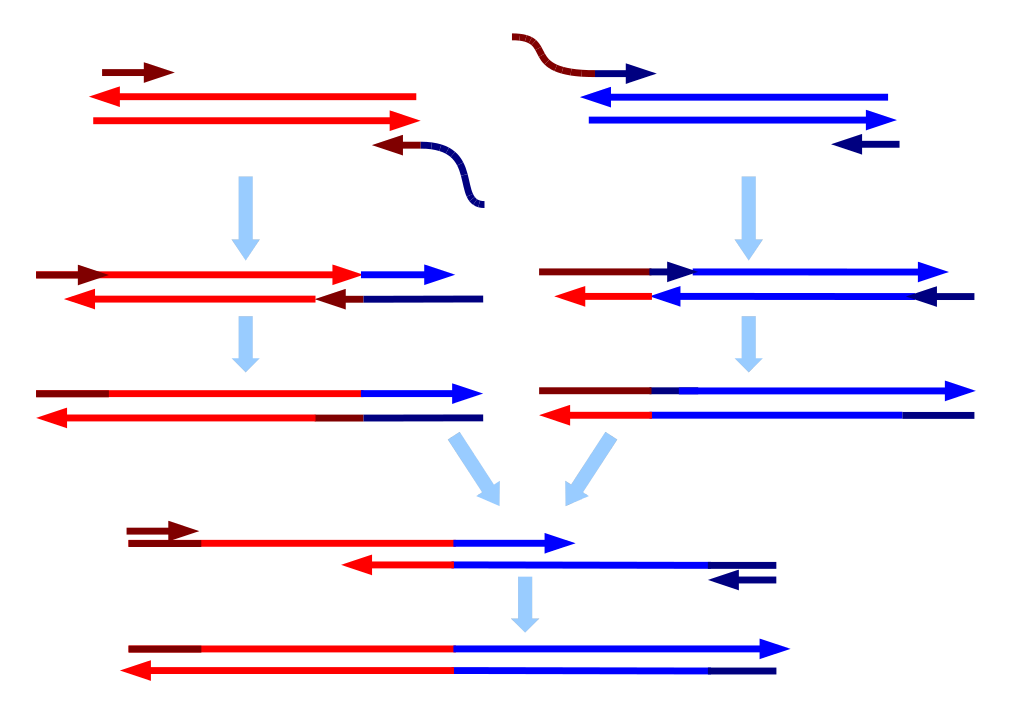
Chimeras
Like the mythical creatures these are named for, sequence chimeras are DNA (or cDNA) strands which are accidentally created when two other DNA strands merged. Chimeric sequences can be made up of more than two DNA strand parents, but the probability of that is much lower. Chimeras occur during PCR, which takes one strand of genetic code and makes thousands to millions of copies, and a process used in nearly all sequencing workflows at some point. If there is an uneven voltage supplied to the machine, the amplification process can hiccup, producing partial DNA strands which can concatenate and produce a new strand, which might be confused for a new species. These can be removed during analysis by comparing the first and second half of each of your sequences to a reference database of sequences. If each half matches to a different “parent”, it is deemed chimeric and removed.
During DNA or RNA extraction, genetic code can be flicked from one sample to another during any number of wash or shaking steps, or if droplets are flicked from fast moving pipettes. This can be mitigated by properly sealing all sample containers or plates, moving slowly and carefully controlling your technique, or using precision robots which have been programmed with exacting detail — down to the curvature of the tube used, the amount and viscosity of the liquid, and how fast you want to pipette to move, so that the computer can calculate the pressure needed to perform each task. Sequencing machines are extremely expensive, and many labs are moving towards shared facilities or third-party service providers, both of which may use proprietary protocols. This makes it more difficult to track possible contamination, as was the case in a recent study using RNA; the researchers found that much of the sample-sample contamination occurred at the facility or in shipping, and that this negatively affected their ability to properly analyze trends in the data.
Sample-sample contamination during sequencing
Controlling sample-sample contamination during sequencing, however, is much more difficult to control. Each sequencing technology was designed with a different research goal in mind, for example, some generate an immense amount of short reads to get high resolution on specific areas, while others aim to get the longest continuous piece of DNA sequenced as possible before the reaction fails or become unreliable. they each come with their own quirks and potential for quality control failures.
Due to the high cost of sequencing, and the practicality that most microbiome studies don’t require more than 10,000 reads per sample, it is very common to pool samples during a run. During wet-lab processing to prepare your biological samples into a “sequencing library”, a unique piece of artificial “DNA” called a barcode, tag, or index, is added to all the pieces of genetic code in a single sample (in reality, this is not DNA but a single strand of nucleotides without any of DNA’s bells and whistles). Each of your samples gets a different barcode, and then all your samples can be mixed together in a “pool”. After sequencing the pool, your computer program can sort the sequences back into their respective samples using those barcodes.
While this technique has made sequencing significantly cheaper, it adds other complications. For example, Illumina MiSeq machines generate a certain number of sequence reads (about 200 million right now) which are divided up among the samples in that run (like a pie). The samples are added to a sequencing plate or flow cell (for things like Illumina MiSeq). The flow cells have multiple lanes where samples can be added; if you add a smaller number of samples to each lane, the machine will generate more sequences per sample, and if you add a larger number of samples, each one has fewer sequences at the end of the run. you have contamination. One drawback to this is that positive controls always sequence really well, much better than your low-biomass biological samples, which can mean that your samples do not generate many sequences during a run or means that tag switching is encouraged from your high-biomass samples to your low-biomass samples.
Cross-contamination can happen on a flow cell when the sample pool wasn’t thoroughly cleaned of adapters or primers, and there are great explanations of this here and here. To generate many copies of genetic code from a single strand, you mimic DNA replication in the lab by providing all the basic ingredients (process described here). To do that, you need to add a primer (just like with painting) which can attach to your sample DNA at a specific site and act as scaffolding for your enzyme to attach to the sample DNA and start adding bases to form a complimentary strand. Adapters are just primers with barcodes and the sequencing primer already attached. Primers and adapters are small strands, roughly 10 to 50 nucleotides long, and are much shorter than your DNA of interest, which is generally 100 to 1000 nucleotides long. There are a number of methods to remove them, but if they hang around and make it to the sequencing run, they can be incorporated incorrectly and make it seem like a sequence belongs to a different sample.
This may sound easy to fix, but sequencing library preparation already goes through a lot of stringent cleaning procedures to remove everything but the DNA (or RNA) strands you want to work with. It’s so stringent, that the problem of barcode swapping, also known as tag switching or index hopping, was not immediately apparent. Even when it is noted, it typically affects a small number of the total sequences. This may not be an issue, if you are working with rumen samples and are only interested in sequences which represent >1% of your total abundance. But it can really be an issue in low biomass samples, such as air or dust, particularly in hospitals or clean rooms. If you were trying to determine whether healthy adults were carrying but not infected by the pathogen C. difficile in their GI tract, you would be very interested in the presence of even one C. difficile sequence and would want to be extremely sure of which sample it came from. Tag switching can be made worse by combining samples from very different sample types or genetic code targets on the same run.
There are a number of articles proposing methods of dealing with tag switching using double tags to reduce confusion or other primer design techniques, computational correction or variance stabilization of the sequence data, identification and removal of contaminant sequences, or utilizing synthetic mock controls. Mock controls are microbial communities which have been created in the lab by mixed a few dozen microbial cultures together, and are used as a positive control to ensure your procedures are working. because you are adding the cells to the sample yourself, you can control the relative concentrations of each species which can act as a standard to estimate the number of cells that might be in your biological samples. Synthetic mock controls don’t use real organisms, they instead use synthetically created DNA to act as artificial “organisms”. If you find these in a biological sample, you know you have contamination. One drawback to this is that positive controls always sequence really well, much better than your low-biomass biological samples, which can mean that your samples do not generate many sequences during a run or means that tag switching is encouraged from your high-biomass samples to your low-biomass samples.
Incorrect base calls
Cross-contamination during sequencing can also be a solely bioinformatic problem – since many of the barcodes are only a few nucleotides (10 or 12 being the most commonly used), if the computer misinterprets the bases it thinks was just added, it can interpret the barcode as being a different one and attribute that sequence to being from a different sample than it was. This may not be a problem if there aren’t many incorrect sequences generated and it falls below the threshold of what is “important because it is abundant”, but again, it can be a problem if you are looking for the presence of perhaps just a few hundred cells.
Implications
When researching environments that have very low biomass, such as air, dust, and hospital or cleanroom surfaces, there are very few microbial cells to begin with. Adding even a few dozen or several hundred cells can make a dramatic impactinto what that microbial community looks like, and can confound findings.
Collectively, contamination issues can lead to batch effects, where all the samples that were processed together have similar contamination. This can be confused with an actual treatment effect if you aren’t careful in how you process your samples. For example, if all your samples from timepoint 1 were extracted, amplified, and sequenced together, and all your samples from timepoint 2 were extracted, amplified, and sequenced together later, you might find that timepoint 1 and 2 have significantly different bacterial communities. If this was because a large number of low-abundance species were responsible for that change, you wouldn’t really know if that was because the community had changed subtly or if it was because of the collective effect of low-level contamination.
Stay tuned for a piece on batch effects in sequencing!
Bioinformatics brings statistics, mathematics, and computer programming to biology and other sciences. In my area, it allows for the analysis of massive amounts of genomic (DNA), transcriptomic (RNA), proteomic (proteins), or metabolomic (metabolites) data.
In recent years, the advances in sequencing have allowed for the large-scale investigation of a variety of microbiomes. Microbiome refers to the collective genetic material or genomes of all the microorganisms in a specific environment, such as the digestive tract or the elbow. The term microbiome is often casually thrown around: some people mistakenly use it interchangeably with “microbiota”, or use it to describe only the genetic material of a specific type of microorganism (i.e. “microbiome” instead of “bacterial microbiome”). Not only have targeted, or amplicon sequencing techniques improved, but methods that use single or multiple whole genomes have become much more efficient. In both cases, this has resulted in more sequences being amplified more times. This creates “sequencing depth”, a.k.a. better “coverage”: if you can sequence one piece of DNA 10 times instead of just once of twice, then you can determine if changes in the sequence are random errors or really there. Unfortunately, faster sequencing techniques usually have more spontaneous errors, so your data are “messy” and harder to deal with. More and messier data creates the problem of handling data.
The grey lines on the right represent sequence pieces reassembled into a genome, with white showing gaps. The colored lines represent a nucleotide that is different from the reference genome, usually just a random error in one sequence. The red bar shows where each sequence has a nucleotide different from that of the reference genome, indicating that this bacterial strain really is different there. This is a single nucleotide polymorphism (SNP).
DNA analysis requires very complex mathematical equations in order to have a standardized way to quantitatively and statistically compare two or two million DNA sequences. For example, you can use equations for estimating entropy (chaos) and estimate how many sequences you might be missing due to sequencing shortcomings based on how homogeneous (similar) or varied your dataset is. If you look at your data in chunks of 100 sequences, and 90 of them are different from each other, then sequencing your dataset again will probably turn up something new. But if 90 are the same, you have likely found nearly all the species in that sample.
Bioinformatics takes these complex equations and uses computer programs to break them down into many simple pieces and automate them. However, the more data you have, the more equations the computer will need to do, and the larger your files will be. Thus, many researchers are limited by how much data they can process.
Mr. DNA, Jurassic Park (1993)
There are several challenges to analyzing any dataset. The first is assembly.
Sequencing technology can only add so many nucleotide bases to a synthesized sequence before it starts introducing more and more errors, or just stops adding altogether. To combat this increase in errors, DNA or RNA is cut into small fragments, or primers are used to amplify only certain small regions. These pieces can be sequenced from one end to another, or can be sequenced starting at both ends and working towards the middle to create a region of overlap. In that case, to assemble, the computer needs to match up both ends and create one contiguous segment (“contig”). With some platforms, like Illumina, the computer tags each sequence by where on the plate it was, so it knows which forward piece matches which reverse.
When sequencing an entire genome (or many), the pieces are enzymatically cut, or sheared by vibrating them at a certain frequency, and all the pieces are sequenced multiple times. The computer then needs to match the ends up using short pieces of overlap. This can be very resource-intensive for the computer, depending on how many pieces you need to put back together, and whether you have a reference genome for it to use (like the picture on a puzzle box), or whether you are doing it de novo from scratch (putting together a puzzle without a picture, by trial and error, two pieces at a time).
Once assembled into their respective consensus sequences, you need to quality-check the data.
This can take a significant amount of time, depending on how you go about it. It also requires good judgement, and a willingness to re-run the steps with different parameters to see what will happen. An easy and quick way is to have the computer throw out any data below a certain threshold: longer or shorter than what your target sequence length was, ambiguous bases (N) which the computer couldn’t call as a primary nucleotide (A, T, C, or G), or the confidence level (quality score) of the base call was low. These scores are generated by the sequencing machine as a relative measure of how “confident” the base call is, and this roughly translates to potential number of base call errors (ex. marking it an A instead of a T) per 1,000 bases. You can also cut off low-quality pieces, like the very beginning or ends of sequences which tend to sequence poorly and have low quality. This is a great example of where judgement is needed: if you quality-check and trim off low quality bases first, and then assemble, you are likely to have cut off the overlapping ends which end up in the middle of a contig and won’t be able to put the two halves together. If you assemble first, you might end up with a sequence that is low-quality in the middle, or very short if you trim it on the low quality portions. If your run did not sequence well and you have lot of spontaneous errors, you will have to decide whether to work with a lot of poor-quality data, or a small amount of good-quality data leftover after you trim out the rest, or spend the money to try and re-sequence.
There are several steps that I like to add, some of which are necessary and some which are technically optional. One of them is to look for chimeras, which are two sequence pieces that mistakenly got joined together. This happens during the PCR amplification step, often if there is an inconsistent electrical current or other technical problem with the machine. While time- and processor-consuming, chimera checking can remove these fake sequences before you accidentally think you’ve discovered a new species. Your screen might end up looking something like this…
Actual and common screen-shot… but I am familiar enough with it to be able to interpret!
Eventually, you can taxonomically and statistically assess your data.
Ishaq and Wright, 2014, Microbial Ecology
In order to assign taxonomic identification (ex. genus or species) to a sequence, you need to have a reference database. This is a list of sequences labelled with their taxonomy (ex. Bacillus licheniformis), so that you can match your sequences to the reference and identify what you have. There are several pre-made ones publicly available, but in many cases you need to add to or edit these, and several times I have made my own using available data in online databases.
Ishaq and Wright, 2014, Microbial Ecology
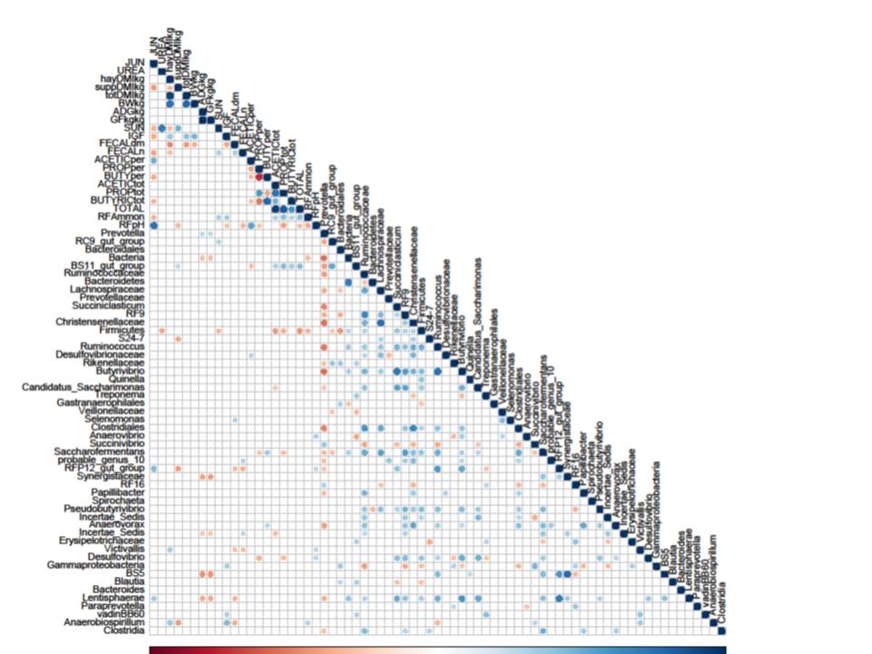
You can also statistically compare your samples. This can get complicated, but in essence tries to mathematically compare datasets to determine if they are actually different, and if that difference could have happened by chance or not. You can determine if organically-farmed soil contains more diversity than conventionally-farmed soils. Or whether you have enough sequencing coverage, or need to go back and do another run. You can also see trends across the data, for example, whether moose from different geographic locations have similar bacterial diversity to each other (left). Or whether certain species or environmental factors have a positive/negative/ or no correlation (below).
Bioinformatics can be complicated and frustrating, especially because computers are very literal machines and need to have things written in very specific ways to get them to accomplish tasks. They also aren’t very good at telling you what you are doing wrong; sometimes it’s as simple as having a space where it’s not supposed to be. It takes dedication and patience to go back through code to look for minute errors, or to backtrack in an analysis and figure out at which step several thousand sequences disappeared and why. Like any skill, computer science and bioinformatics take time and practice to master. In the end, the interpretation of the data and identifying trends can be really interesting, and it’s really rewarding when you finally manage to get your statistical program to create a particularly complicated graph!
Stay tuned for an in-depth look at my current post-doctoral work with weed management in agriculture and soil microbial diversity!